Mouse Coronal Brain and Spinal Cord
Simulation Engine for Creation of Synthetic Microscope Images and Corresponding Labels.
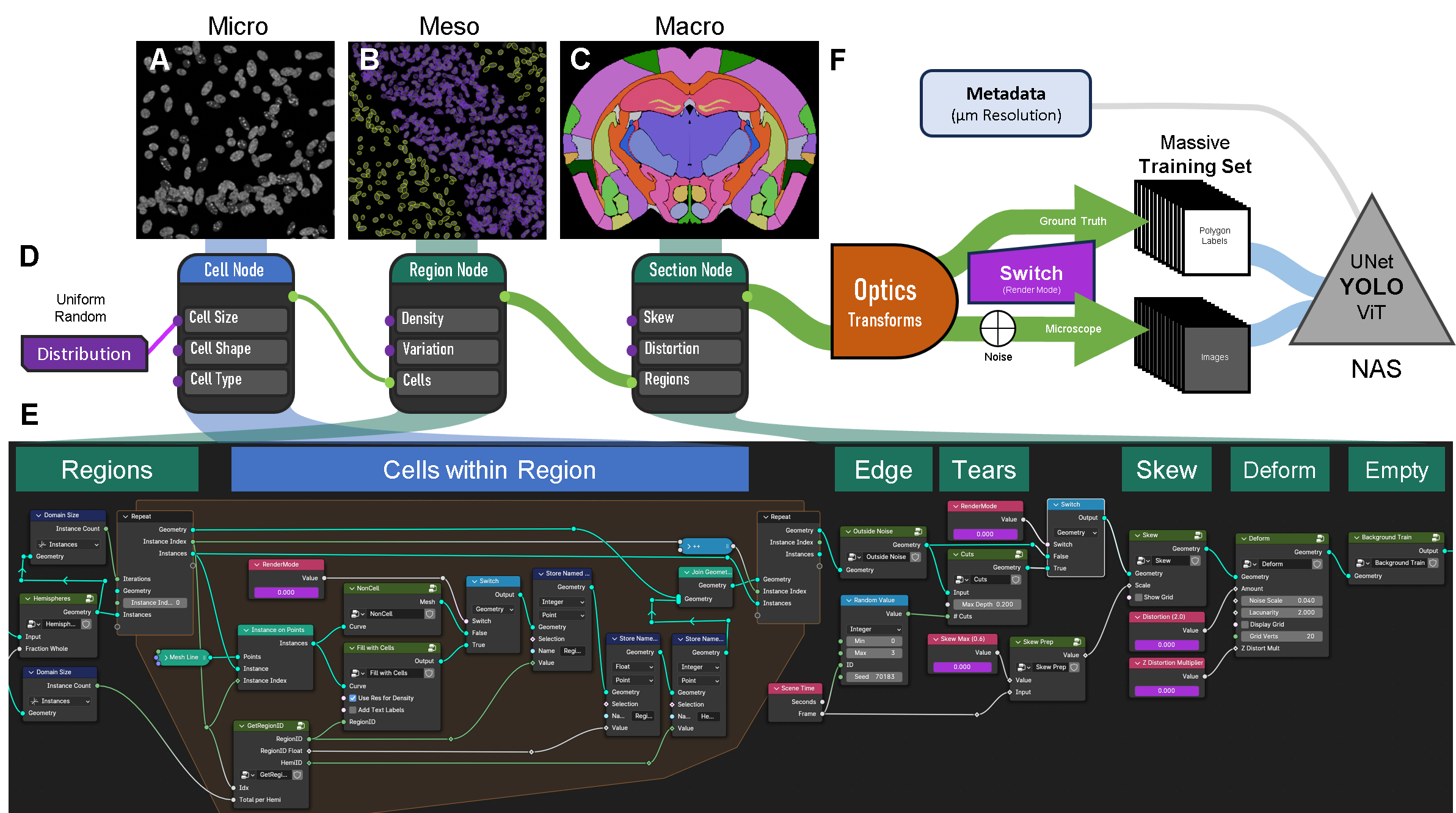
The figure is organized to show the different modules used to produce the datasets for training:
A–C. Micrographs and illustrations of the A) micro-, B) meso-, and C) macro-scale representations of a coronal section of a mouse brain.
D. Three “nodes” represent the main concepts within the engine. These connect to the images above and the Blender Geometry Nodes pipeline that executes each scale. The simulation pipeline starts with uniform random distributions controlling input parameters for Cell, Region, and Section properties. Each input node (circle on the left) lists example parameters (cell size, shape, type). Each output node (green circle on the right) passes 3D geometry to the next node. The connections between nodes increase in diameter, showing growing geometric complexity.
E. The Geometry Nodes pipeline within Blender that produces coronal brain and spinal cord simulations. Polygon regions from an atlas are inputs. A central repeat zone (orange background) iterates through regions. The center of each iteration defines cell geometry. Section parameters include Edge (debris and cells at boundaries), Tears (rips or tears), Skew and Deform (distortions), and Empty (occasional blank/background scenes).
F. Created geometry is passed through an optics/physics engine to generate images. Each image set includes a ground-truth version and a microscope-like version. A workflow switch changes parameters across the pipeline, adding noise at the end. Images are rendered with corresponding polygons and labels. Metadata (pixel resolution and full settings) is also saved. These datasets are then used to train a neural network, typically YOLO instance segmentation with neural architecture search (NAS).
How to use
- Open above linked dile in Blender ≥ 4.4.
- Choose either Coronal or Spinal Collection
- In the Scene Properties, set the parameter values (see table below).
- Go to the Geometry Nodes tab on the top, and examine, edit the geometry settings as desired.
- Go to the script tab on the top. There you will see a script called bla hbla.
- Adjust the # of images to render, and the destination, then Run the script.
Troubleshooting
- If there are problems, experiment with moving to different frames, and adjusting the parameters.
- Slow renders. There is also code in the script that allows the rendering to happen from command line, this is at least twice as fast.
Simulation Parameters (in Scene Properties)
| Simulation Parameter | Default Value | Notes |
|---|---|---|
| FIVCellDensityVarianceFactor | 3.5 | 1 = no Cell Density variance between regions, higher the number, more cell density variance. This is ignored if CurveRes_forDensity is selected. |
| FIVDensityFactor | 12 | Multiplier that increases the overall density. Older brains or larger organisms need more cells per region, but ~12 is good for adult mouse. |
| FIVFractionWhole | 0.05 | 1 = All renders are a complete brain, 0 = all renders are hemisections, anything inbetween gives different proportions of whole vs hemisections. |
| FIVSizeFactor | 0.35 | The size of the nuclei/cell within each region. |
| FIV_CurveRes_forDensity | FALSE | When TRUE, the density of each region can be encoded into the CurveResolution parameter of each object. |
| FIV_DistortionAmount | 1.2 | Maximum Distortion Factor. 0 to keep all renders un-distorted. |
| FIV_MaxCompositorNoise | 0.94 | Each render has varying amounts of noise added to the final image in the compositing step. 0 removes the noise, 1 means only noise. |
| FIV_SkewAmount | 0.2 | Maximum amount of skew, where 0 disallows any skew. |
| FIV_Z_DistortionMultiplier | 1 | Additional multiplier for distortions, only works if DistortionAmount is > zero. |
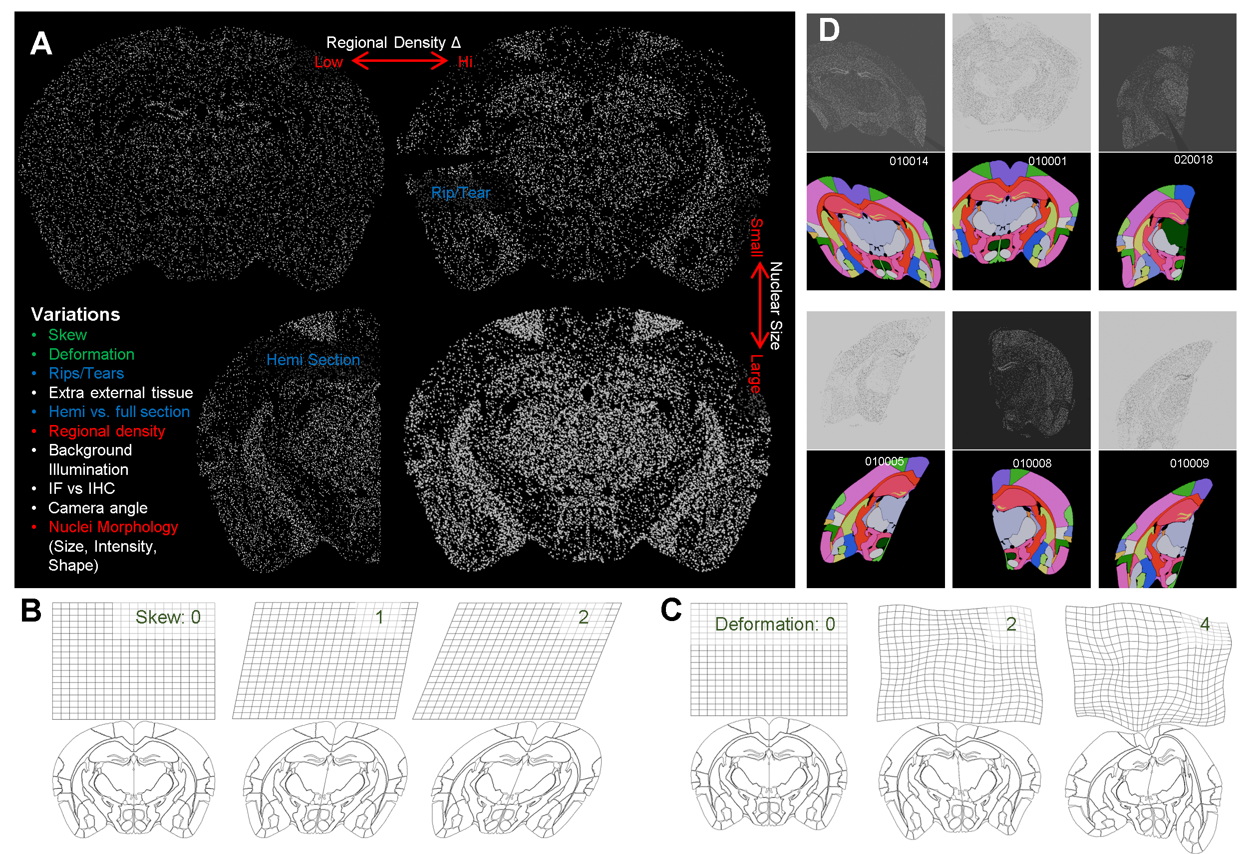
Mouse Brain Macro simulation generation.
A. Overview of the different variations we can model using Blender Geometry Nodes.
B. Skew moves the orientation of the plane of slice relative to the microscope, representing different slice angles, where 2 is a more extreme example.
C. Deformation mimcs the natural variation observed in the shape of the slices between individuals..
D. Examples of rendered macro images with different levels of variations with their respective labels. The white text is the image’s unique ID.
Script used to Render and Export training dataset.
From within the .blend file (linked above), go to the scripting tab along the top, and find this script "Export Script". You will notice several parameters you can set, importantly, where to save (base_path), and how many images to render (start_ and end_frame). Press play when ready to trigger the rendering and the label production.
Dense Nuclei
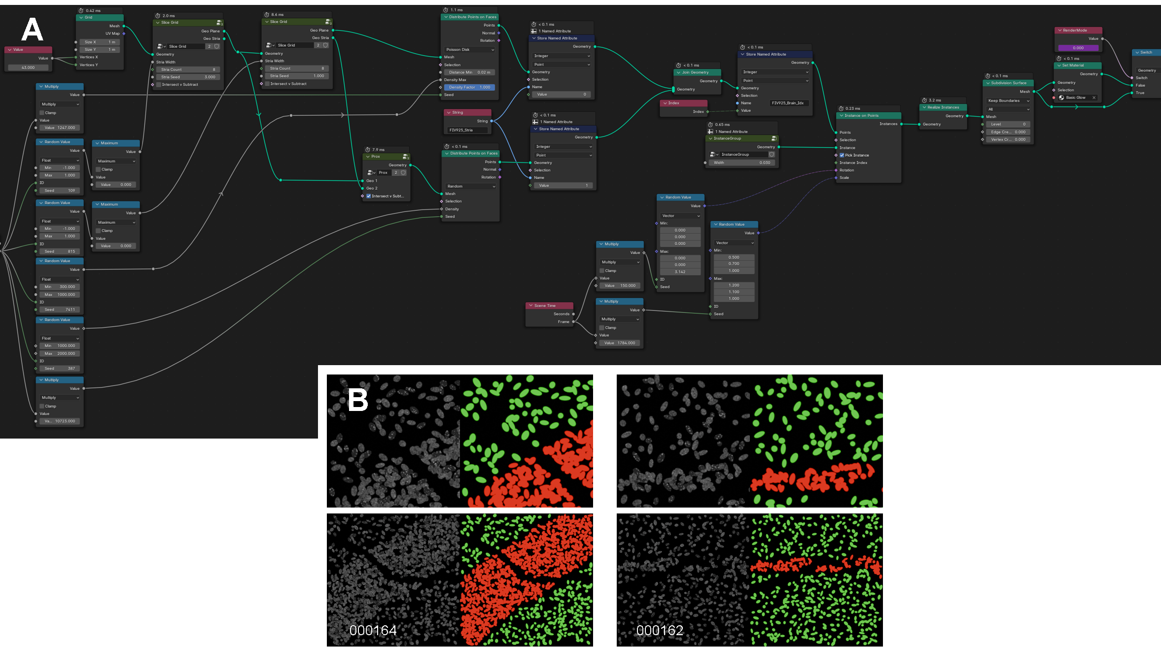
Micro Model GeoNodes and Simulation Examples.
A. Geometry nodes used to generate the micro- and meso-scale image sets of the central nervous system.
B. Examples of rendered meso-scale images. In white text is the image’s unique ID. Each colored image is the label for the respective image to its left. The bottom row is a more zoomed out version of the row above to better demonstrate the tissue striations. Green represents adjacent cells; red represents high density stria or bands of cells.
Peripheral Nerve Fascicles
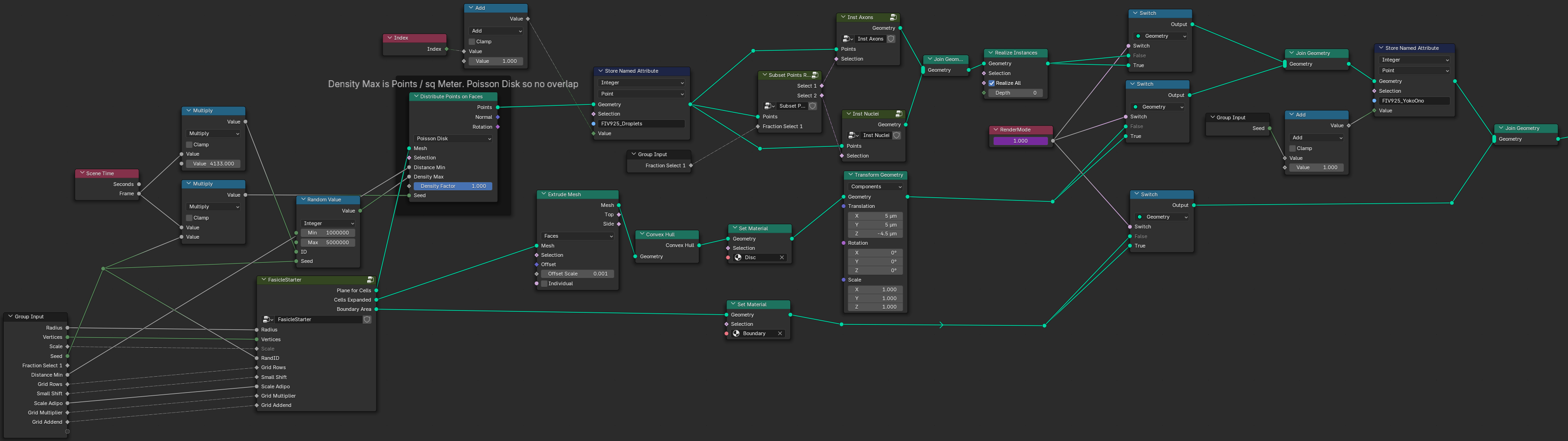
Blender GeoNodes tree producing Fascicle Training sets.
View of the Blender Geometry Nodes tree which is used to control synthetic fascicle production. Pressing tab on any of the groups (such as "Fascicle Starter") will go inside of this nodegroup and show additional nodes and links.
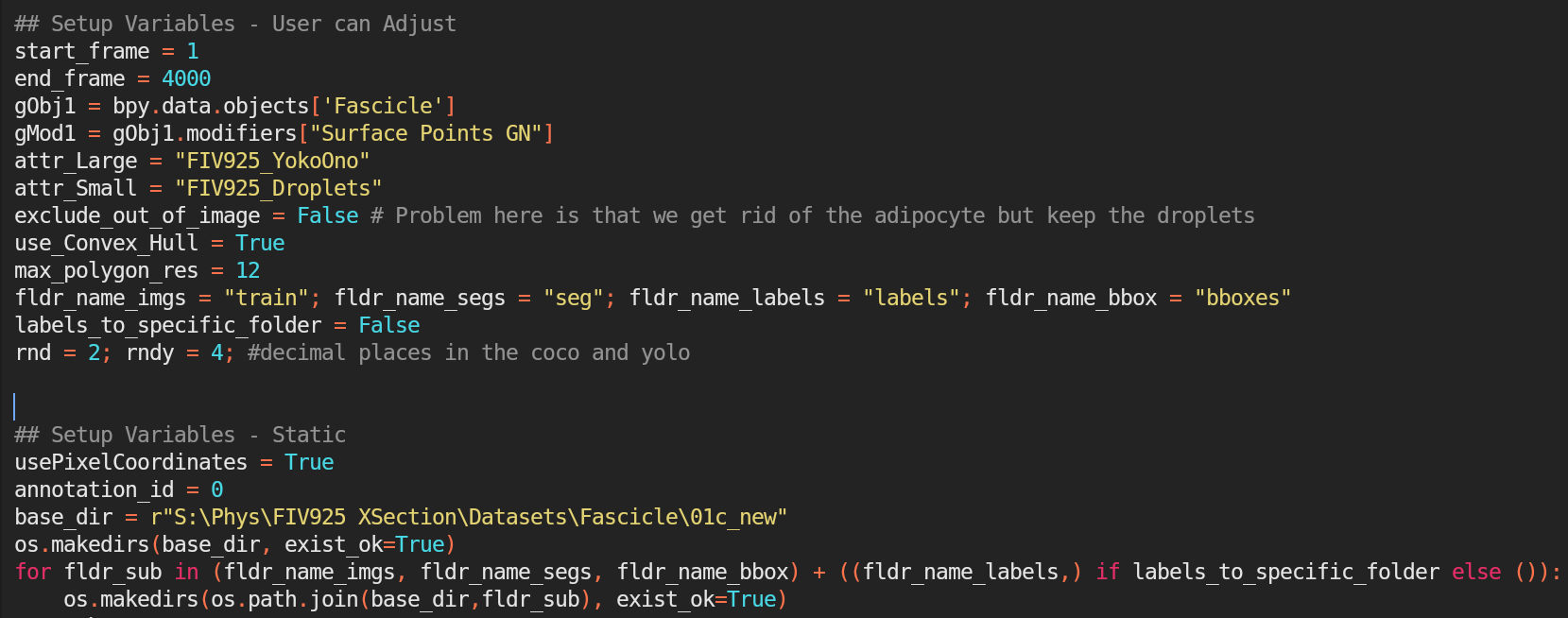
Script to render Fascicles.
On the "Scripting" tab on the top of Blender, find the "Export Script", and use it to render the images and labels. Notice several variables including base_dir and start/end_frame that can be adjusted.